LDC User Guide¶

REVISION HISTORY¶

Revision No.	Description	Date
1.0	Initial release	07/13/2022
1.1	Add description of Rotate parameter	06/19/2022

1. OVERVIEW¶

1.1. Basic Conception¶

LDC (Lens Distortion Correction) is an image processing technique used to correct lens distortion. Lens distortion is a phenomenon where the image is distorted due to the optical characteristics of the lens. By applying LDC, the image undergoes geometric correction, making it more aligned with human visual expectations.

1.1.1. Field Angle¶

Used to describe the field of view of a picture, It can be divided into horizontal field Angle αand vertical field Angle β.

For a lens with distortion, the field Angle will have a larger field Angle due to the optical relationship of lens refraction.

Figure 1-1 Without distortion

Figure 1-2 With distortion

The movement of the field of view is manifested as the change of the picture content, and the movement of the field of view will not change the size of the field of view, it is a process of rotating around the optical center.

Figure 1-3 Moving the field of view horizontally to the right

Figure 1-4 Moving the field of view horizontally to the upwards

1.1.2. Barrel Distortion¶

The closer to the corner, the more the image extends outward, the more severe the distortion, visually causing the barrel-shaped effect of the middle arch.

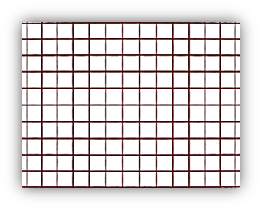
Figure without distortion

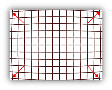
Figure with barrel distortion

1.1.3. Pincushion Distortion¶

The closer to the corner, the more the image extends outwards and forwards, the more severe the distortion is, visually causing the effect of a depression in the middle.

Figure without distortion

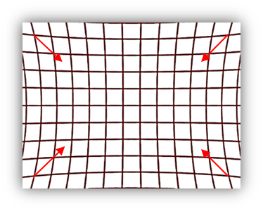
Figure with pincushion distortion

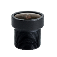
1.1.4. Len¶

The lens is an important optical device of the camera, its light transmittance, focal length, field of view, distortion, etc. will directly affect the overall effect of the image. Table 1-1 describes some of its characteristics and recommended correction modes for the LDC function.

Table 1-1 Recommendations for Lens Correction Modes
lens type	sample	description
distortion-free lens		Distortion is negligible, no distortion correction required.
Wide-angle lens		With a certain degree of distortion, it has a wider field of view. Because the field of view is not large enough, 360°/180° panorama correction cannot obtain a good field of view effect. It is recommended to use Normal correction to eliminate distortion.
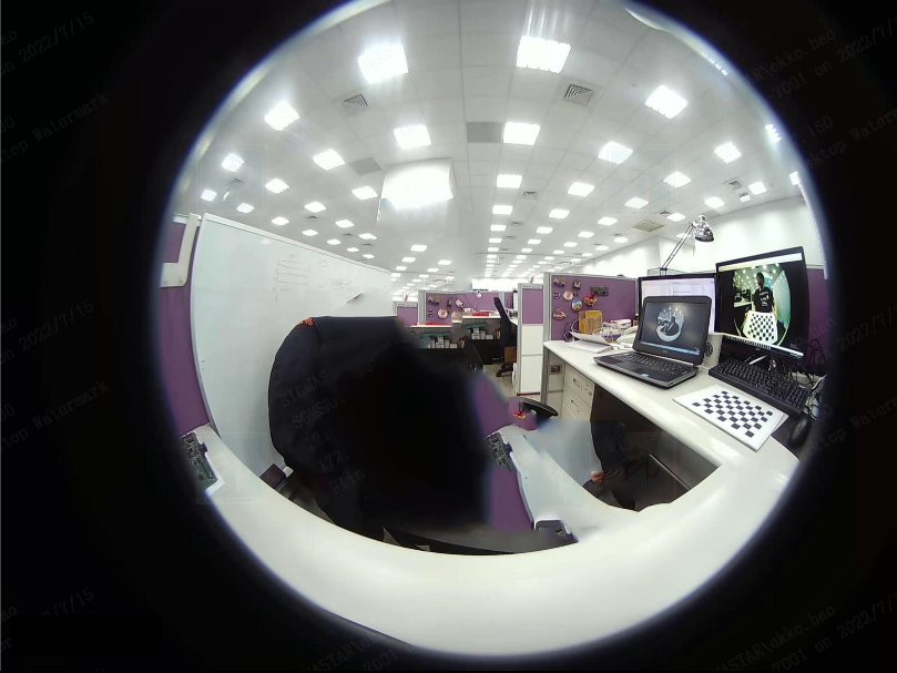
Fisheye lens		The field of view is extremely large and can cover the entire field of view plane, but the degree of distortion is relatively large. You can use the 180°/360° panorama correction mode to process the picture to get more views, or use the multi-region Normal correction mode for processing.

1.1.5. Invalid Image Area¶

The invalid area refers to the area beyond the pixel range of the original image when LDC combs to generate the output image, for example, the field of view is moved out of the field of view of the original image by simulating the movement of the field of view. Invalid areas will be filled with black color.

Figure for Invalid Image Area

1.1.6. Drawing Region¶

Output image We can regard it as an output screen, on which we can draw the image processed by the LDC module in the specified region according to actual needs. Intersection, tangency, and separation between the drawing areas are all available.The width and height alignment limits of the region are consistent with the screen. For example, the width alignment of the screen requires 16 pixels, and the width of the region also requires 16 pixels of alignment.

Table 1-2 Drawing regions interrelationships and effects
Relationships between regions	Effect
Intersect	The region with a large serial number (drawn later) will cover the image of the overlapping area.
Separate	Hollow areas will be drawn with the background color
Tangent	The images of each region are displayed separately. No hole areas. No overlapping areas.

Figure 1-6 is used to display the view relationship of the drawing region. The black part is a hollow area, which can be filled with freely configurable background color.

Figure 1-6 The view relationships of drawing region

2. Development Guide¶

2.1. Basic parameters¶

For the LDC function, it is necessary to configure some basic parameters for the normal output of the function, as shown in Table 2-1.

Table 2-1 LDC basic parameter configuration
RegionAttr	Description		Range
RegionMode	The used LDC function for the current region
	360 ° panorama correction	Distortion correction function Refer to Chapter 2.2 for detailed parameter configuration	1
	180° panorama correction		2
	Normal correction		3
	Mapping table schema (Map2bin)	Refer to Chapter 2.3 for detailed parameter configuration	4
	bypass mode (No Transformation)	Refer to Chapter 2.5 for detailed parameter configuration	5
OutRect	Select an area in the output image to draw the output image of the current region. This parameter is not to configure the final output image size, but the output size of the current region. If you want only one output and the output covers the screen, the width and height can be configured to be equal to the size of the final output image. s After configuring the width and height, LDC will scale the output image of the current region to this size.
	X	The abscissa of the upper left corner of the drawing region	[0, out_w]
	Y	The vertical coordinate of the upper left corner of the drawing region	[0, out_h]
	Width	The width of drawing region	[0, out_w - X]
	Height	The height of drawing region	[0, out_h - Y]
RegionNum	The number of drawing regions After configuring the value of region number, you need to configure the functions and detailed parameters of each region within this value, and you do not need to configure the region exceeding this value.		(0, 9]
BgColor	Background color configuration. color format is RGB888. When the configuration of this parameter is enabled, the background color of the output screen will be configured as the specified color, such as green rgb(0,255,0) = 0x0000FF00 When the configuration of this parameter is disabled, the background color of the screen will be black rgb(0,0,0)= 0x0000000		[0x0, 0xFFFFFF]

2.2. Lens Distortion Correction¶

2.2.1. Mode Description¶

Lens Distortion Correction mode, the MI LDC module corrects through the lens Calibration information (CalibInfo) and the correction method specified by the user, and performs cropping as required, zooming and outputting to the specified area.

2.2.2. Flowchart¶

Figure 2-1 Distortion correction mode usage process

2.2.3. Camera Installation¶

The installation of the camera supports three installation modes: ground installation, ceiling installation, and wall installation. Its characteristics and typical scene examples are shown in Table 2-2:

Table 2-2 Camera installation method and description of its features
Mount mode	Description
Desktop mount (DM)	The camera is installed in the scene where the upward viewing angle is expected, such as on the ground, on the table, etc.
Ceiling mount (CM)	The camera is installed in the scene where the bird's-eye view is desired, such as on the ceiling or on the roof, etc.
Wall mount (WM)	The camera is installed in scenes where a head-up view is desired, such as between buildings or courtyard walls, etc.

Different installation methods and correction modes are not bound one by one. In actual use, you can choose the matching correction mode to achieve the best view and effect.

2.2.4. Correction mode and parameter description¶

360 °panorama correction:

Table 2-3 Description of 360-degree panorama correction parameters
Typical Scene	ceiling mount, desktop mount
Parameter Description	Pan	The starting position of the correction area in the circumferential direction relative to the original image; Affects the left border of the output image.
	Tilt	The starting position of the correction area in the radial direction relative to the origin of the original image; Affects the upper border of the output image.
	ZoomH	The end position of the correction area in the circumferential direction relative to the original image; Affects the right border of the output image.
	ZoomV	The end position of the correction area in the radial direction relative to the original image; Affects the lower border of the output image.
Corrective Model

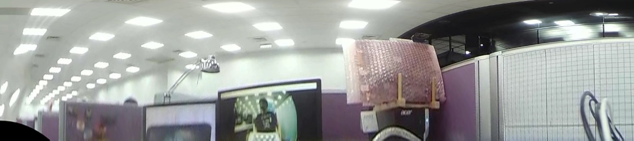
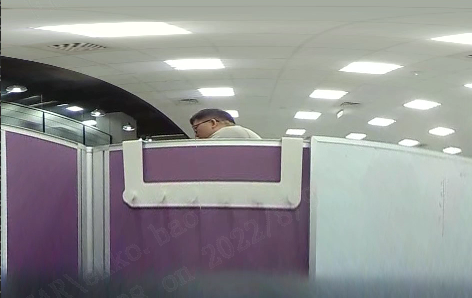
180° panorama correction:

Table 2-4 Description of 180-degree panorama correction parameters
Typical Scene	wall mount
Parameter Description	Pan	The field of view is rotated left and right, which is used to simulate a camera rotation left and right.
	Tilt	The field of view is rotated up and down, which is used to simulate a camera rotation up and down.
	ZoomH	The size of the horizontal field of view; Affects the horizontal field of view of the output image.
	ZoomV	The size of the vertical field of view; Affects the vertical field of view of the output image.
	Rotate	Simulate a camera rotation.
Corrective Model

Normal Correction:

Table 2-5 Description of Normal correction parameters
Typical Scene	Wall mount, Ceiling mount, Desktop mount
Parameter Description	Pan	The field of view rotated left and right, which is used to simulate a camera rotation left and right.
	Tilt	The field of view rotated up and down, which is used to simulate a camera rotation up and down.
	ZoomH	Adjust the size of the field of view (horizontal & vertical). Affects the overall field of view of the output image.
	ZoomV	Invalid parameter, no configuration required.
	Rotate	Simulate a camera rotation.
Corrective Model

2.2.5. Application scenarios and parameter configuration instructions¶

Ceiling Mount, Desktop Mount:

When the camera is installed on the top or the ground, it is recommended to use the 360-degree correction mode or the Normal correction mode.

The parameter description and range of 360-degree correction mode are shown in Table 2-6.
The parameter description and range of Normal correction mode are shown in Table 2-7.

Table 2-6 360-degree correction parameter configuration instructions
Parameter	Description		Parameter range
Pan	The starting position of the correction area in the circumferential direction relative to the original image; Unit: angle		ZoomH > Pan ZoomH – Pan <= 360
Tilt	The starting position of the correction area in the radial direction relative to the center point of the original image; Unit: pixel		[InRadius,OutRadius]
ZoomH	The end position of the correction area relative to the original image in the circumferential direction; For an area spanning 0° (360°), for example, extending 270° to 45°, use (Pan=270°,ZoomH=360°+45°=405°) is enough. Unit: angle		ZoomH > Pan ZoomH – Pan <= 360
ZoomV	The end position of the correction area in the radial direction relative to the center point of the original image; Unit: pixel		[InRadius,OutRadius]
InRadius	The radius from the border to the center point in the maximum valid area in the original image. If set to 0, it will take effect as 1; If it exceeds FisheyeRadius, it is equal to FisheyeRadius Unit: pixel		(0,FisheyeRadius]
OutRadius	In the original image, the radius from the outer boundary of the maximum effective area to the center point. If set to 0, it will take effect as 1; If it exceeds FisheyeRadius, it is equal to FisheyeRadius Unit: pixel		(0,FisheyeRadius]
MountMode	must be Ceiling mount or Desktop mount.		0,1
	0	Desktop mount
	1	Ceiling mount

Table 2-7 Description and range of Normal correction parameters
Parameter	Description		Parameter Range
Pan	Simulate the left and right rotation of the camera, which affects the field of view position of the output image. Equal to boundary value if out of bounds. Unit: angle		[-90,90]
	= 0	no rotation
	< 0	turn left
	> 0	turn right
Tilt	Simulate the up and down rotation of the camera to affect the field of view position of the output image. Equal to boundary value if out of bounds. Unit: angle		[-90,90]
	= 0	no rotation
	< 0	turn down
	> 0	turn up
ZoomH	Adjust the size (scale) of the field of view (horizontal & vertical). Affects the overall field of view of the output image. Equal to boundary value if out of bounds.		[0,500]
	= 100	no adjustment
	> 100	Narrows the field of view and sees less images, but at the expense of image quality.
	< 100	The field of view is widened to see more images, but it will bring invalid areas.
ZoomV	invalid parameter
Rotate	Simulate the rotation of the camera. Unit: angle		[0,360]
	= 0	no rotation
	> 0	Rotate counterclockwise, 360 is a circle.
MountMode	The configuration can be Ceiling mount, Desktop mount, or Wall mount.		0、1、2
	0	Desktop Mount
	1	Ceiling Mount
	2	Wall Mount

Wall Mount:

When the camera is wall-mounted, it is recommended to use 180-degree correction mode or Normal correction mode.

The parameter description and range of 180-degree correction mode are shown in Table 2-8.
The parameter description and range of Normal correction mode are shown in Table 2-7.

Table 2-8 Parameter description and range of 180-degree correction mode
Parameter	Description		Parameter range
Pan	Simulate the left and right rotation of the camera, which affects the field of view position of the output image. Equal to boundary value if out of bounds. Unit: angle		[-90,90]
	= 0	no rotation
	< 0	turn left
	> 0	turn right
Tilt	Simulate the up and down rotation of the camera, which affects the field of view position of the output image. Equal to boundary value if out of bounds. Unit: angle		[-90,90]
	= 0	no rotation
	< 0	turn down
	> 0	turn up
ZoomH	Adjust the size of the horizontal field of view. Equal to boundary value if out of bounds.		[0,500]
	= 100	no adjustment
	> 100	Narrows the field of view and sees less images, but at the expense of image quality.
	< 100	The field of view is widened to see more images, but it will bring invalid areas.
ZoomV	Adjust the size of the vertical field of view. Equal to boundary value if out of bounds.		[0,500]
	= 100	no adjustment
	> 100	Narrows the field of view and sees less images, but at the expense of image quality.
	< 100	The field of view is widened to see more images, but it will bring invalid areas.
Rotate	Simulate the rotation of the camera. Unit: angle		[0,360]
	= 0	no rotation
	> 0	Rotate counterclockwise, 360 is a circle.
MountMode	must be wall mount.		2
MountMode	2	wall mount	2

The configuration of the parameters in the above respective modes has different effects in the corresponding modes. The following is the description of the common parameters, which have the same effect on each correction mode.

Table 2-9 Common parameters of distortion correction
Parameter	Description		Parameter range
OutRotate	Rotate the output graph around the center Unit: angle		[0,360]
	= 0	no rotation
	> 0	Rotate counterclockwise, 360 is a circle.
DistortionRatio	Reduce the strength of distortion correction to improve the field of view. Not suitable for 360° panorama correction.		[-100,100]
	= 0	No adjustment of correction strength
	> 0	Correction strength for reducing barrel distortion. The larger the absolute value is, the stronger the attenuation effect will be, resulting in larger image distortion and larger viewing angle. Too large to form pincushion distortion.
	< 0	Correction strength for reducing pincushion distortion. The larger the absolute value is, the stronger the attenuation effect will be, resulting in larger image distortion and larger viewing angle. Too large to cause barrel distortion.
FocalRatio	Change the virtual focal length. By changing this parameter, the distance between the image and the projection surface can be adjusted to achieve the effect of pushing/pulling the image without losing the field of view. If set to 0, it will take effect as 10000. Not suitable for Normal correction.		(0,50000]
	= 10000	no adjustment
	> 10000	The larger the value, the smoother the picture and the smaller the curvature.
	< 10000	The smaller the value, the more curved the screen and the greater the curvature.
CropMode	Invalid region detection and cropping are performed on the output image to eliminate invalid regions. If the output image is all invalid areas, an error will be reported if the value is not 0, so you can configure other parameters first, and then configure this parameter according to the need after confirming that the output image meets expectations.		0,1,2
	0	Do not perform invalid area detection, output according to the original output image.
	1	Use the largest effective area of the screen, and stretch to form the same aspect ratio as the original output image. This method can obtain the largest effective area but the picture may be distorted.
	2	Keep the aspect ratio of the original output image, frame the maximum effective area, and then enlarge it to the size of the output image. This method can ensure that the picture will not be deformed but may lose the field of view.
CalibInfo	Len Infomation
CalibPolyBin	Lens distortion information data. Generated by the LDC Tool on the PC side, set when setting the LDC channel properties, the data must match the actual lens used. Otherwise, the effect of distortion correction will be affected.
CenterXOffset CenterYOffset	The offset between the CMOS center point and the lens center point can be used to eliminate the deviation caused by the assembly of the lens center point and the CMOS center point. Unit: pixel		Configuration beyond the image range will result in invalid area output.
	0	no offset
	> 0	The center of the screen is located to the right/below of the image center
	< 0	The center point of the screen is on the left/upper side of the image center point
FishEyeRadius	Lens radius, used to describe the radius of the entire effective frame in the image Fisheye lens: configured as the effective picture radius Wide-angle lens: configured as half of the effective screen diagonal		Matching with lens distortion information

2.2.6. Example of 360-degree panorama correction effect¶

Table 2-10 Examples of different parameters for 360-degree panorama correction
Parameter setting		Correction effect
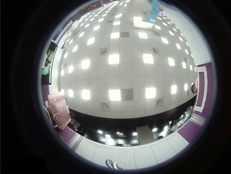
srcWidth	1600	Fisheye Input Image 1600x1200 The center point of the effective picture relative to the image is closer to the upper right, resulting in the lack of some content above it
srcHeight	1200
MountMode	0
CenterXOffset	75
CenterYOffset	-34
FishEyeRadius	620
InRadius	0
OutRadiusght	600
FocalRatio	10000
CropMode	0
Parameter sequence 1
Pan	0	Expand the entire original image from the inside to the outside to form the effect of a panoramic expanded image. The blurred line at the lower boundary corresponds to the edge area of the fisheye lens, and the missing part above the original image is displayed as a black invalid area in the output image.
ZoomH	360
Tilt	0
ZoomV	600

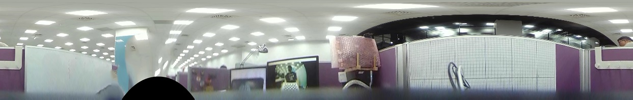
360 °panorama corrected output image 3768x600
Parameter sequence 2
Pan	0	Relative to parameter sequence 1: Reduce ZoomV (far away from the outer boundary of the fisheye), and remove the blurred part of the edge. Increase the tilt (away from the center of the fisheye) to remove the more stretched part of the upper boundary.
ZoomH	360
Tilt	100
ZoomV	520

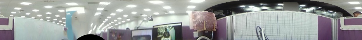
360 °panorama corrected output image 3768x420
Parameter sequence 3
Pan	90	Only correct for footage between 90 and 270 degrees Comparing with the parameter sequence 2, it can be seen that 1/4 of the picture on the left and right sides has been removed, and the upper and lower boundaries remain unchanged.
ZoomH	270
Tilt	100
ZoomV	520

360 °panorama corrected output image 1884x420
Parameter sequence 4
Pan	315	Expand the frame between 315° and 405°, which is equivalent to -45° to 45°. (Pan)->(ZoomH) == (Pan-360°) ->(ZoomH-360°)
ZoomH	405
Tilt	100
ZoomV	600

360 °panorama corrected output image 942x600

2.2.7. Example of 180-degree panorama correction effect¶

Table 2-11 Examples of different parameters for 180-degree panorama correction
Parameter setting		Correction effect
srcWidth	1600	Fisheye Input Image 1600x1200 The effective picture is relatively up and right relative to the center point of the image, resulting in the loss of part of the content above it.
srcHeight	1200
MountMode	2
CenterXOffset	75
CenterYOffset	-34
FocalRatio	10000
CropMode	0
Parameter sequence 1
Pan	0		No up and down rotation, no scaling of field of view. The renderings are as follows.
Tilt	0
ZoomH	100
ZoomV	100
FishEyeRadius	620

1600x1200
Parameter sequence 2
Pan	0	Compared with the parameter sequence 1, the value of FishEyeRadius is reduced, and the blurred border image is removed to improve the effect.
Tilt	0
ZoomH	100
ZoomV	100
FishEyeRadius	580

1600x1200
Parameter sequence 3
Pan	0	Compared with the parameter sequence 2, the horizontal and vertical field of view are changed, the places with large edge stretching are removed, and the values of the two are adjusted according to the image effect.
Tilt	0
ZoomH	120
ZoomV	200
FishEyeRadius	580

1300x600
Parameter sequence 4
Pan	0	Compared with parameter sequence 1, change the tilt to adjust the position of the camera angle of view. Turn down 50°, form a top-down perspective.
Tilt	-50
ZoomH	100
ZoomV	100
FishEyeRadius	620

1600x1200 The lower black part of the output image is caused by the FishEyeRadius setting being too large. Reducing the FishEyeRadius can eliminate the black area. If the FishEyeRadius setting is too large and exceeds the effective range of the original image, an invalid area will be generated.
Parameter sequence 5
Pan	-50	Compared with the parameter sequence 4, adjust the Pan parameter again, so that the camera rotates 50° to the left and rotates 50° to the down.
Tilt	-50
ZoomH	100
ZoomV	100
FishEyeRadius	620

1600x1200

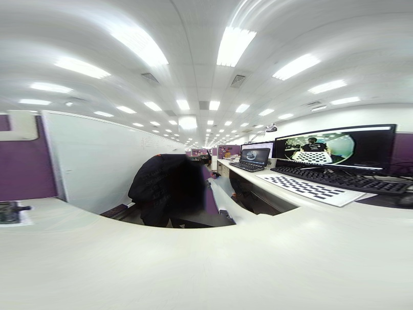
2.2.8. Example of Normal correction effect¶

Table 2-12 Example of Normal correcting the effect of different parameters
Parameter
srcWidth	1600	Fisheye input image with resolution 1600x1200 The center point of the effective picture relative to the image is closer to the upper right, resulting in the lack of some content above it.
srcHeight	1200
MountMode	2
CenterXOffset	75
CenterYOffset	-34
Rotate	0
CropMode	0
Parameter sequence 1
Pan	0		No up and down rotation, no zooming of field of view.
Tilt	0
ZoomH	100

1600x1200 It can be seen from the renderings that compared with 180° panorama correction, the objects in the picture are less stretched and bent (light strips), and are linear and radial, but the field of view is smaller.
Parameter sequence 2
Pan	0	Compared with parameter sequence 1, change the value of tilt to make the camera rotate downward by 50°.
Tilt	-50
ZoomH	100

1600x1200 From the effect point of view, compared with the panoramic correction parameter sequence 4, the field of view is smaller, but the physics is more straight (checkerboard).
Parameter sequence 3
Pan	-50	Compared with parameter sequence 2, the Pan value is changed. Make the camera turn left 50°, and turn down 50°.
Tilt	-50
ZoomH	100

1300x600
Parameter sequence 4		Compared to parameter sequence 1, the value of ZoomH is changed.
Pan	0
Tilt	0
ZoomH	200	Compared with ZoomH = 100, the center content is zoomed in and the field of view is narrowed
ZoomH	100	Default effect
ZoomH	50	Compared with ZoomH = 100, its center content is pushed away, radially outward along the center point, and the more the edge is visually stretched, the stronger it is. The black arc area above is an invalid area, because some content exceeds the valid area of the original image.
Parameter sequence 5
Pan	0	Modify the value of Rotate to simulate camera rotation. In wall mounted scenes, the correction image must be positive and has no effect when both Pan and Tilt are 0.
Tilt	32
MountMode	2
Rotate	0	No rotation
Rotate	90	The correction area has been rotated 90 degrees
Rotate	270	The correction area has been rotated 270 degrees
Parameter sequence 6
Pan	0	Compared to parameter sequence 5, change the camera to ground mounted.
Tilt	32
MountMode	0
Rotate	0	No rotation
Rotate	90	The correction area has been rotated 90 degrees, and the image has also been rotated 90 degrees
Rotate	270	The correction area has been rotated 270 degrees, and the image has also been rotated 270 degrees

2.2.9. Examples of other parameter effects¶

Example of CropMode

Table 2-13 Example of CropMode
Input Image
CropMode = 0 Output the original image after correction	Output Image
CropMode = 1 Frame the maximum effective area and scale it adaptively to the size of the output image	Crop Effect	Output Image
CropMode = 2 Frame the effective area according to the ratio of the output image, and then zoom in proportionally to the size of the output image	Crop Effect	Output Image

Example of FocalRatio

Table 2-14 Example of FocalRatio
FocalRatio = 2000	Compared with FocalRatio = 10000, the lens is zoomed in, the center object is released, and it is clearer; the edge objects are compressed, and the picture is more curved (refer to the edge of the desktop)
FocalRatio = 10000	Default Effect, only perform 180° panorama correction on the original image
FocalRatio = 20000	Compared with FocalRatio = 10000, the lens is zoomed out, the content in the center is compressed, the edge objects are released, and the picture is smoother (refer to the edge of the desktop)

Example of OutRotate

Table 2-15 Example of OutRotate
OutRotate = 0	Default effect, only perform 180° panorama correction on the original image
OutRotate = 45	du Rotate 45° counterclockwise. The output image is not rotated here, but the area corresponding to the output is rotated in the original image. If the area corresponding to the rotated output image does not exceed the area of the original image, no invalid area (black area) will be generated

Example of DistortionRatio (barrel distortion)

Table 2-16 Example of DistortionRatio
DistortionRatio = -10	Strengthen the correction effect, the edge of the desktop is straighter, but the overall field of view is narrowed
DistortionRatio = 0	Default Effect
DistortionRatio = 10	Weaken the correction effect, the edge of the desktop is more curved, but the overall field of view is wider

2.3. Displacement Map Mode¶

2.3.1. Description¶

Displacement map Mode (also called MAP2BIN), A special mode provided for the convenience of users to directly use LDC hardware to realize customized LDC functions.

When the Region is in this mode, the MI LDC module will receive the input and output image mapping data set by the user, convert it into data that can be processed by the LDC hardware according to the user's map, and hand it over to the hardware to complete the construction of the output image.

Displacement map: Store the pixel coordinate mapping from the output image to the input image, divided into Xmap and Ymap, which record the pixel coordinates of the input image (x_in,y_in) corresponding to the pixel coordinates of each output image (x_out,y_out)

2.3.2. Flowchart¶

Table 2-2 Usage of Displacement Map Mode

2.3.3. Parameter Configuration Description¶

Table 2-17 Parameter Description of Displacement Map Mode
Parameter	Description	Parameter range
Grid	In order to improve processing performance, maps are usually after downsampling. In order to reduce the amount of calculation, not every pixel is included in the map, but the interpolation operation is performed during hardware processing to restore it. The Grid parameter was introduced at this time to describe the sampling interval (accuracy) For example, a 3840x2160 output image, its original map is 3840x2160, in the case of grid = 16, the map width is reduced to 241x136	1,2,4,8,16,32,64
Xmap Ymap	Divided into x-coordinate mapping table and y-coordinate mapping table. Store the horizontal and vertical coordinate values of the corresponding coordinates according to the sampling points The point P in the output image corresponds to the coordinate point P1 of the original image, and the coordinate relationship stored in the map buff is as follows: Due to the downsampling, not every point needs to be calculated, just calculate according to the Grid step; if the pixels at the end cannot divide the Grid, you need to expand or truncate to the actual boundary according to the actual situation. For the difference detail, please refer to Item 1 in Section 2.3.6.	NA
XmapSize YmapSize	The data type of each element in the Map data buff is float type, and the size is 4 bytes. To calculate the width and height of the map here, it needs to be rounded up to ensure that the pixels at the end are included For example, if a 3840x2160 output image has Grid = 16, the buff size occupied by a single map is 214x136x4=131104(bytes), or algo will throw an error.	NA

2.3.4. Example of Map Generation¶

Example map of input-output image is 1:1

The resolution of the processed input image is 1920x1080, Grid = 16, it's width = 1080/16 = 67.5, and truncated to 1080. Map width and height will be 121x69, Example as 2-18.

Table 2-18 Example of 1:1 Map
row/col	0	1	2	…	118	119	120
0	0, 0	16, 0	32, 0	…,0	1888,0	1904,0	1919,0
1	0,16	16,16	32, 16	…,16	1888,16	1904,16	1919,16
2	0,32	16,32	32,32	…,32	1888,32	1904,32	1919,32
…	0,….	16,…	32,…	...,…	1888,…	1904,…	1919,…
…	0, ….	16,…	32,…	...,…	1888,…	1904,…	1919,…
66	0,1056	16,1056	32,1056	…,1056	1888,1056	1904,1056	1919,1056
67	0,1072	16,1072	32,1072	…,1072	1888,1072	1904,1072	1919,1072
68	0,1079	16,1079	32,1079	…,1079	1888,1079	1904,1079	1919,1079

2.3.5. Parameter configuration examples and effects¶

The following is a map with EIS anti-shake and additional fine changes in the lower right corner.

Its required parameters are shown in 2-19:

Table 2-19 Example of Map Mode
Parameter		Description
RegionMode	4	Mode of MI_LDC current Region
srcWidth	1920	input image size 单位：pixel
srcHeight	1080	input image size 单位：pixel
dstWidth	1920	Output Image Size Unit：pixel
dstHeight	1080	Output Image Size Unit：pixel
Grid	16	Sampling accuracy
XmapSize	33396	The memory size required by map Unit: bytes
YmapSize	33396	The memory size required by map Unit: bytes

The mapping diagram of its xymap and the comparison of its input and output diagrams used on the board are shown in Table 2-20.

Table 2-20 Effect of Map
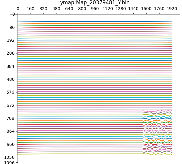
Xmap	Ymap
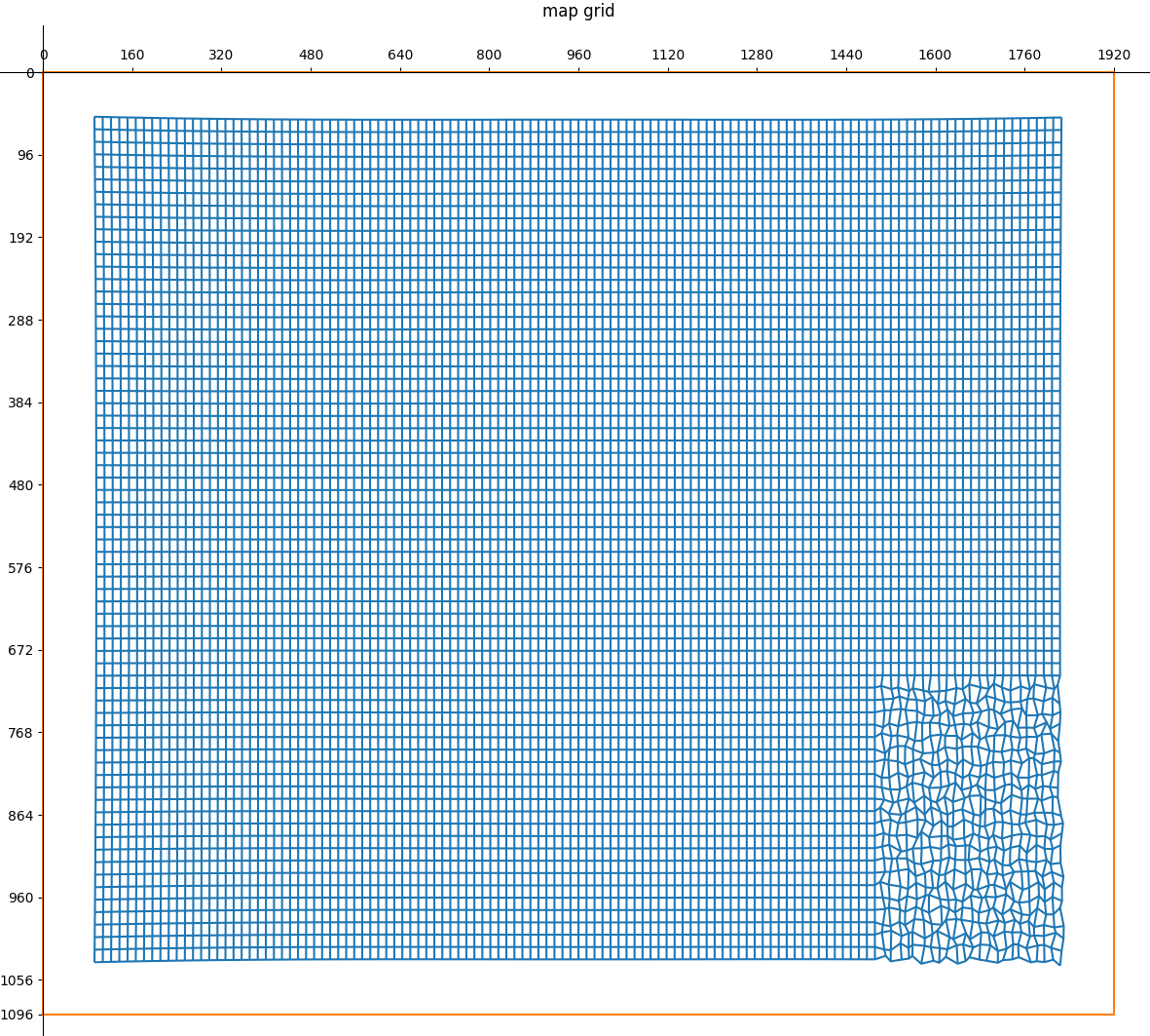
Input and output mesh graph
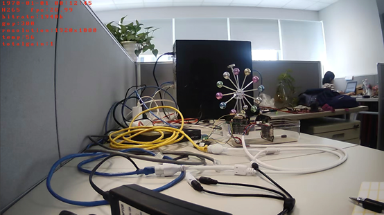
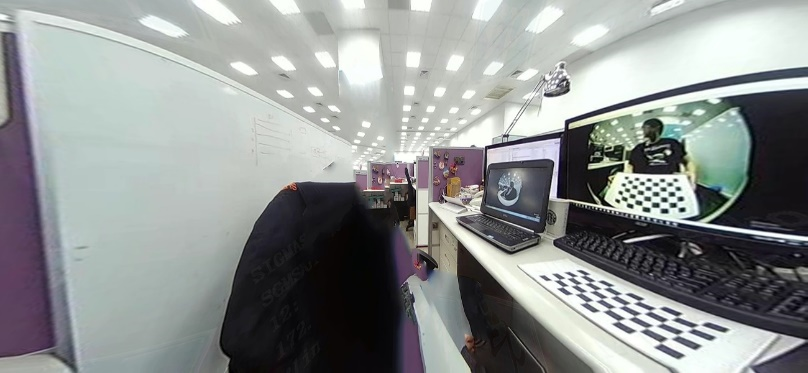
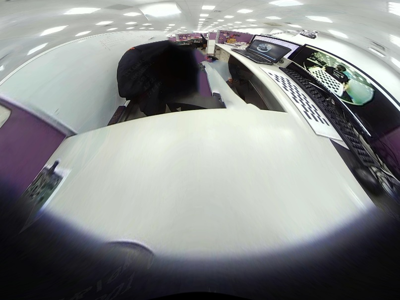
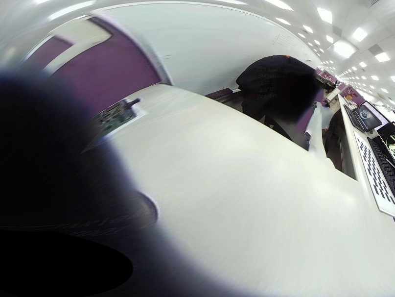
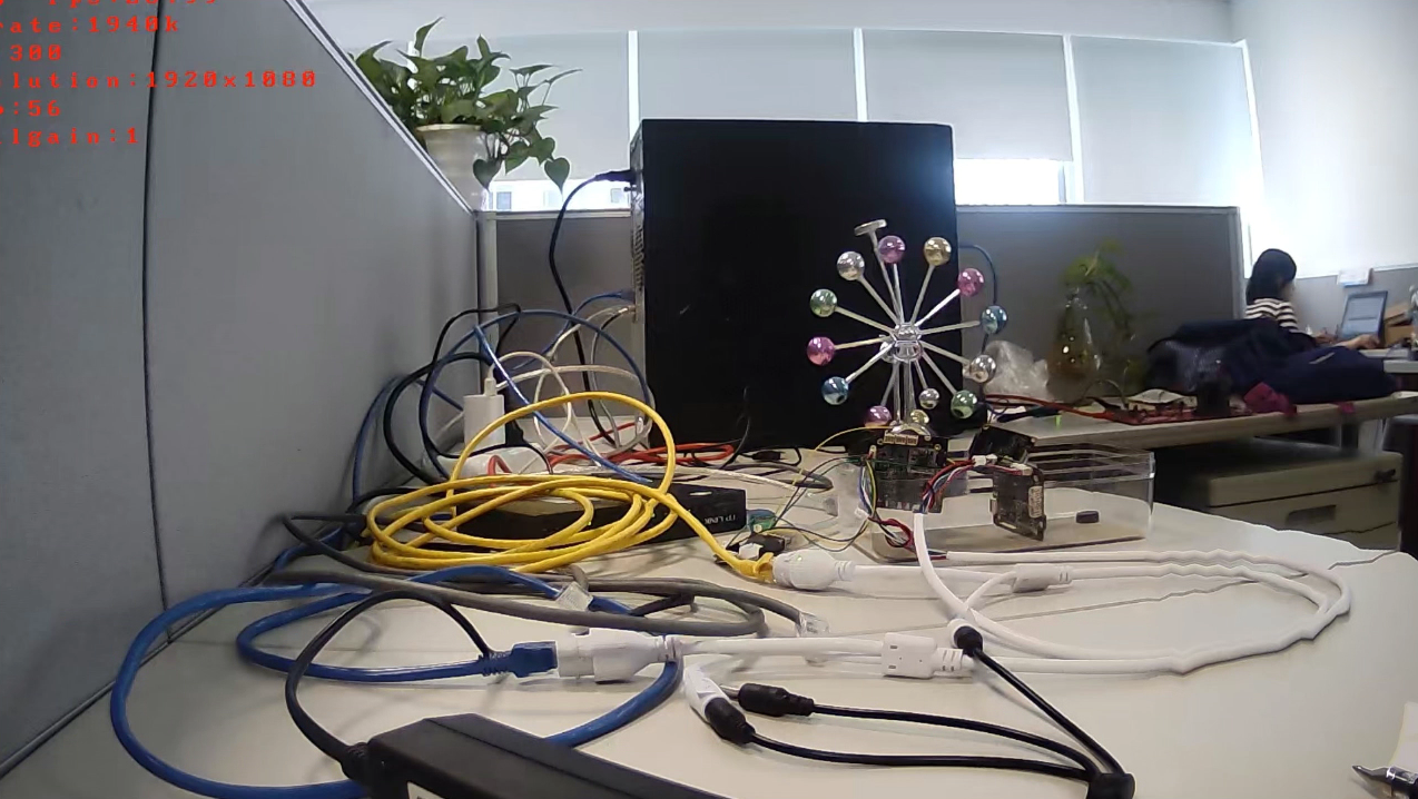
Input Image	Output Image
Input and output comparison chart Obviously, it is consistent with the effect shown in the map shown above.

2.3.6. Map Specifications and Limitations¶

The following situations will occur if the width and height of the image cannot be divisible by Grid. It will result in black borders with map expanded according to the Grid.

SrcImage: 1920x1080 Map range: 1920x1088
Input Image
Output Image

If it is truncated to the boundary, stretching at the boundary will occur, resulting in the problem of missing some pixels.

SrcImage: 1920x1080 Map range: 1920x1080
Input Image
Output Image	The yellow ones with a white background under the pen holder are closer to the boundary relative to the input image

This situation is a hardware limitation, so it is recommended to use a resolution that can be divisible by Grid as input.

Limits on map complexity:
Due to hardware limitations, the entire image cannot be processed at one time, so the image needs to be divided into multiple regions for sequential processing. And the limitations of dividing this processing area are as follows:

The maximum y value of each row minus the minimum y value of the previous row cannot exceed 128 pixels. If the change of the map is too large or the grid is too large and the accuracy is too low to be processed, you can reduce the Grid to improve the sampling accuracy and see if it can be processed.

2.4. Projection Mapping Function¶

2.4.1. Description¶

The user can use Projection Mapping Function (PMF) completing the plane geometric change of the image by configuring the projection transformation matrix, and generate the corresponding output image.

Common types of plane geometric transformations are: translation, rotation, scaling, perspective. Each transformation can be superimposed on each other, and the process of superposition is matrix point multiplication.

Figure 2-3 Schematic diagram of scene projection transformation

Rigid transformation: translation, rotation
Linear transformation: scaling, shear, rotation
Affine transformation: linear, rigid
Projective transformation: affine, perspective

The output image generation process is to operate the pixel coordinates and the specified 3x3 matrix to obtain the corresponding coordinate points in the input image.

The formula is as follows：

2.4.2 Flowchart¶

Figure 2-4 Flowchart of PMF

2.4.3 Matrix usage instructions¶

This matrix (m33) describes the mapping relationship from output coordinates to input coordinates. The corresponding relationship between each item and projection transformation is shown in Figure 2-5.

For different projection transformations, the values of the items will affect each other, so it is generally necessary to calculate the transformation matrix through tools. Only simple single transformations can be achieved with manual adjustments.

Figure 2-5 Schematic diagram of item and effect relationship

The calculation method of the matrix is as follows:

The calculation of the matrix can be divided into the following types according to the requirements. Note that the matrix template provided here is the mapping from the input image to the output image (xy->uv), and the result directly calculated according to this template needs to find its inverse matrix (uv ->xy) to be used as the value of m33~origin of the API.
1. Translation matrix template: Translate Δy rightward (right is positive) and downward (down is positive), along the origin.

2. Rotation matrix template: Rotate θ degrees counterclockwise around the origin (upper left corner of the input image).

3. Scaling matrix template: Scale the image horizontally by Scalex times and vertically by Scaley times (which can realize mirror and flip effects).

4. Shear matrix template: Skews the image by α degrees along the horizontal axis and β degrees along the vertical axis.

5. Perspective matrix template: Perspective matrix needs to obtain the transformation matrix through the four points of the target plane and the coordinates in the current image.

The use of m33_origin matrix (uv->xy) needs to go through two steps: quantization and fixation. The operation is as follows:

Quantization:
Among them, m_8 is the quantization factor. After calculating the initial M33, each item needs to be divided by m_8 to obtain the quantized M33^'.

2. Fixation:
For the convenience of use, each m33 needs to be fixed-pointed, and converted into a fixed-point number with a precision of 1/(2²⁵) for representation. The fixed-point rules are as follows, and each item can be multiplied by 2²⁵.

2.4.4 Parameter Description¶

Table 2-21 Example of PMF Parameter Configuration
Parameter	Description	Parameter range
as64PMFCoef	1. Used to store the m33 matrix after quantization + fixed point 2. The elements m_n in m33 are stored in as64PMFCoef according to the subscript	m_0	[-67108864,67106816]
		m_1	[-67108864,67106816]
		m_2	[-137438963472, 137434759168]
		m_3	[-67108864,67106816]
		m_4	[-67108864,67106816]
		m_5	[-137438963472, 137434759168]
		m_6	[-32768,32767]
		m_7	[-32768,32767]
		m_8	33554432

2.4.5 Example of Parameter Configuration¶

The calculation process from an instance of PMF M33_origin (uv->xy) to API parameters is:

Quantize it and pinpoint it:



The parameter as64PMFCoef finally set in the interface is:

2.4.6 Single transformation example¶

Table 2-22 Some examples of single transform effects for PMF
Translation transformation
Input Image with resolution 800x800
Pan 200pixel right, 100pixel down Origin m33 (uv->xy)： as64PMFCoef：
Rotation transform:
Rotate 10° counterclockwise around the origin. Origin m33 (uv->xy)： as64PMFCoef：
Scale transformation
The horizontal axis is reduced to the original 0.5, and the vertical axis is expanded to the original 1.5 Origin m33 (uv->xy)： as64PMFCoef：
Shear transformation
Shear 15° in the horizontal axis direction and 5° in the vertical axis direction Origin m33 (uv->xy)： as64PMFCoef：
Perspective transformation
Restore the skewed checkerboard plane to vertical The coordinates of the four corners of the image are: (244,139),(770,141),(765,613),(213,605) The four points mapped onto the new output plane are: (244,139),(770,139),(770,599),(244,599) Origin m33 (uv->xy)： as64PMFCoef：

2.4.7 Composite Transformation Calculation Example¶

A complex effect can be obtained by disassembling and combining multiple transformations. The superposition of a single effect can be obtained by dot multiplication of matrices. The usage can be divided into the following steps:
1. Confirm the target effect, that is, what the final effect is, and break it down into sub-steps. Each sub-step can be accomplished with the basic matrix listed above.
2. Generate the matrices of the sub-steps separately.
3. Carry out the point multiplication operation of the matrix according to the sub-step in reverse order. (Note that the commutative law does not apply to matrix multiplication, and the order cannot be changed at will.)
4. Find the inverse matrix of the output m33 (LDC needs the mapping matrix from the output image to the input image), and change it into m33 of nv->xy.
5. Perform quantization and fixation process according to the scheme of the parameter configuration example above, to get the parameter that can be used by the LDC API.

Note:
1. Regarding the two "perspectives" of matrix operations in images (coordinate system unchanged and image unchanged), we use the perspective based on unchanged coordinate system to understand and split the sub-steps.
2. All operations are based on the coordinate origin (the upper left corner of the image), so if you want to implement any operation that centers on a certain point, you need to use a translation matrix to move the center point of the operation to the origin, and move back when the operation is finished.

Case 1:
Rotate the image center by 45 degrees: you need to use a translation matrix and a rotation matrix. The stacking order of the effects is:
Step0. Move the center point of the image to the origin of the coordinates (the rotation matrix uses the origin as the rotation center).
Step1. Rotate the image 45° counterclockwise.
Step2. Move the center point of the image back to the center point of the coordinate.
The correlation matrix is as follows:

m33_origin_comb (xy->uv)

The matrix calculation process is as follows:
Step2 · Step1 · Step0

m33_origin (xy->uv)

Then calculate the inverse matrix of the calculated matrix, and perform quantization and fixed-point summing to set it to MI API for use:

Calculate m33_origin (xy->uv) to obtain m33_api (uv->xy)

Input and output effects obtained by rotating 45 degrees around the center

Case 2:
Mirror the image: you need to use a scaling matrix and a translation matrix. The stacking order of the effects is:
Step0. Use the scaling matrix to change the image to x=-x, y=y, forming a mirror effect with the Y axis as the symmetrical axis.
Step1. Move the image to the right into the coordinate system.
Its correlation matrix is as follows:

m33_origin_comb (xy->uv)

The process of calculating the matrix to obtain the parameters of the API is as follows:

(Step1 · Step0)^-1 -> Quantization and fixation:

Calculate m33_origin (xy->uv) to obtain m33_api (uv->xy)

Mirror effect of input and output diagram

2.5. LDC Bypass Mode¶

2.5.1. Description¶

Working in bypass mode (No Transformation), the current region will not perform distortion correction processing, including lens distortion correction, mapping tables, etc., but supports rotation and adaptive scaling of the output image (when the output and input resolutions are inconsistent,the input is scaled to the output resolution) operate

2.5.2. Flowchart¶

Figure 2-6 LDC Flow chart of bypass mode

2.5.3. Parameter Description¶

Table 2-23 Parameter Description of LDC Bypass Mode
Parameter	Description		Range
OutRotate	Rotate the output graph around the center Unit: angle		[0,360]
	= 0	no Rotation
	> 0	Rotate counterclockwise, 360 is a circle

2.5.4. Example of parameter effects¶

Table 2-24 Example of LDC Bypass Mode Parameter Effects
Input Image with resolution 1600x1200
Adaptive scaling to the output image	Output Image with resolution 1920x1080
OutRotate = 45	Output Image with resolution 1600x1200

2.6. LDC DoorBell Mode¶

2.6.1. Description¶

Working in doorbell mode, it allows users to dynamically adjust five parameters: Fx (X-direction correction force), Fy (Y-direction correction force), A (X-direction compression), B (Y-direction compression), and Scale (image scaling) to observe the effect of correction output.

2.6.2. Flowchart¶

Figure 2-7 LDC Flow chart of DoorBell

2.6.3. Parameter Description¶

Table 2-25 Parameter Description of DoorBell
Parameter	Description
Fx	Horizontal correction strength, value range: [0, 2000]. The final setting value is Fx*0.001.
Fy	Vertical correction strength, value range: [0, 2000]. The final setting value is Fy*0.001.
A	Horizontal scaling, value range: [1000, 4000]. The final setting value is A*0.001.
B	Vertical scaling, value range: [1000, 4000]. The final setting value is B*0.001.
Scale	Output scaling, value range: [200, 20000]. The final setting value is Scale*0.001.

2.6.4. Example of parameter effects¶

Table 2-26 Example of DoorBell Mode Parameter Effects
Parameter		Input Image	Output Image
Example 1
Fx	1000
Fy	1000
A	1000
B	1000
Scale	1850
Example 2
Fx	1500
Fy	1500
A	1000
B	1000
Scale	1200

3. Calibration tool¶

The CV Tool user manual is released together with the SDK and can be found in the Tools directory. Please refer to the user manual inside.