6. IPU Performance Analysis
1. IPU Performance Analysis
1.1 Viewing Offline Model Information
The tool for viewing offline model information: SGS_IPU_Toolchain/DumpDebug/show_img_info.py.
(1) Command to use the tool:
python3 show_img_info.py \
-m deploy_fixed.sim_sgsimg.img \
--soc_version chip_model
(2) Required parameters:
-m, --model: Path to the offline model.
--soc_version: Chip model.
The output will display the following information:
Explanation
-
Offline IMG Version: The version information of the SDK used to generate this offline model from the dataset. -
Offline Model Size: The size of this offline model in bytes. -
Offline Model Max Batch Number: The maximum batch size of this offline model. (Compiler tool-b, --batchparameter) -
Offline Model Suggested Batch: A suggested batch size that can be referenced in the model, which can be set to any batch size less than or equal to the Max Batch Number during actual use. (Compiler tool--batch_modeparameter) -
Offline Model Supported Batch: The available batch sizes for the one_buf model. Only these batch sizes can be selected. (Compiler tool--batch_modeparameter) -
Offline Model Variable Buffer Size: The size of the Variable Buffer needed by the offline model, in bytes. -
Offline_Model:-
Input:name: The name of the model input tensor.
index: The index of the model input tensor.
dtype: The data type of the model input tensor,
uint8orallint16.layouts: The data layout of the model input tensor,
NCHWorNHWC.shape: The shape information of the model input tensor.
training_input_formats: The image format information used during the network training (input_config
training_input_formatsparameter).input_formats: The image input format for the network model when running on chips (input_config
input_formatsparameter).input_width_alignment: The number of alignment in the width direction when the data is used as network input (input_config
input_width_alignmentparameter).input_height_alignment: The number of alignment in the height direction when the data is used as network input (input_config
input_height_alignmentparameter).batch: The batch size of this offline model.
batch_mode: The batch mode of the model, either
n_buforone_buf. -
Output:name: The name of the model output tensor.
index: The index of the model output tensor.
dtype: The data type of the model output tensor,
uint8orallint16.shape: The shape information of the model output tensor.
batch: The batch size of this offline model.
batch_mode: The batch mode of the model, either
n_buforone_buf
-
1.2 Viewing IPU Performance
The Linux SDK-alkaid provides the app located at sdk/verify/release_feature/source/dla/dla_dla_show_img_info.
Executing the prog_dla_dla_show_img_info executable on the board can print and view the model’s performance data.
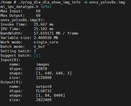
Explanation
Invoke Time: The time taken by the Invoke API on the board. The Invoke API time includes: CPU driver IPU working time,IPU Time, synchronization time for model output data to DRAM, etc.IPU Time: The time cost for IPU hardware.BandWidth: The amount of data accessed from DRAM during one model execution.Variable size: The runtime memory requested by the model. Multiple models can share this memory, so the largestVariable sizeamong the models needs to be selected.work_mode: Information about the model's single-core or dual-core mode.Batch mode: Information about the model's batch mode.Setting batch: The batch value set during the conversion of the offline model.Suggest batch: The batch value contained internally in the offline model.
1.3 IPU Log Performance Analysis
The IPU Log performance analysis tool is located at SGS_IPU_Toolchain/Scripts/example/performance_timeline.py. Passing the generated IPU Log during model execution into the parsing script will generate a json formatted file in the current directory. Open Google Chrome and type chrome://tracing, then drag the generated json file into the browser to visualize it.
1.3.1 Running Offline Models to Generate IPU Log
The Linux SDK-alkaid provides the app located at sdk/verify/release_feature/source/dla/dla_dla_show_img_info.
Executing the prog_dla_dla_show_img_info executable on the board generates the ipu_log, including binary files ending with _core0.bin, _core1.bin, and _corectrl0.bin.
./prog_dla_dla_show_img_info \
-m deploy_fixed.sim_sgsimg.img \
--ipu_log logdir
Parameter explanations:
-m, --model: The path to the offline model.
--ipu_log: The directory for saving the generated IPU log.
Note
-
If the buffer size of the IPU Log is insufficient, you will see an error in the serial output or via
dmesg, as shown in the red box below. The generated IPU Log will be incomplete; you need to increase the--ipu_log_sizeparameter to regenerate the IPU Log.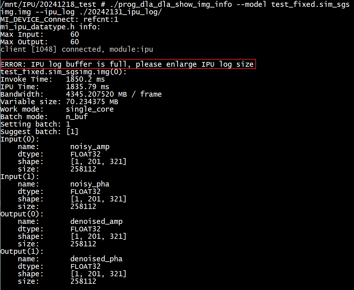
-
The information printed during the generation of IPU Log, such as Invoke Time, IPU Time, and Bandwidth, should not be trusted. Please collect the printed data when not generating IPU Log as performance information of the model.
1.3.2 How to Generate a JSON File from IPU Log
python3 ~/SGS_IPU_Toolchain/Scripts/example/performance_timeline.py \
-c0 log_core0.bin \
-c1 log_core1.bin \
-cc log_corectrl0.bin \
-f 900 \
-v muffin
Parameter explanations:
-c0, --core0: The path to the core0 IPU log file (only require the core0 IPU log for single-core).
-c1, --core1: The path to the core1 IPU log file.
-cc, --corectrl: The path to the corectrl IPU log file (optional).
-f, --frequency: The IPU clock frequency (default is 800).
-v, --ipu_version: The IPU chip version (e.g., muffin).
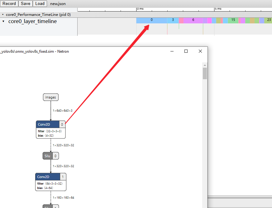
After execution, a log_ctrl0.json file will be generated in the running directory. Drag the generated JSON file into the Google Chrome browser at chrome://tracing to display the performance time percentage for each layer, with the following explanation of the terms:
Term
- start: The start time of this layer.
- wall duration: The time taken for this layer.
- total_cycle: The number of cycles for this layer, which can be converted to "wall duration" as wall duration = total_cycle/freq.
- conv_cycle_percent: The percentage of this layer's convolution runtime relative to the total runtime of this layer.
- vector_cycle_percent: The percentage of this layer's vector runtime relative to the total runtime of this layer.
- dma_load_cycle_percent: The percentage of this layer's DMA load runtime relative to the total runtime of this layer.
- dma_store_cycle_percent: The percentage of this layer's DMA store runtime relative to the total runtime of this layer.
- Convolution, vector, DMA load, and DMA store instructions can execute in parallel, so the percentage sum may not equal 100%.
1.3.3 How to Use the Tool to Statistically Analyze Operator Execution Time
python3 ~/SGS_IPU_Toolchain/Scripts/DumpDebug/get_op_time_cost.py \
-m /path/to/fixed.sim \
--ipu_log_file /path/to/log.json
Parameter explanations:
-m: Pass in the fixed.sim model.
ipu_log_file: Pass in the JSON file generated in Section 1.3.2.
mode: Supports two modes: each and total, with the default being total.
In total mode, it prints the time percentage for each operator type. Once finished, the terminal will print the time percentages for each type of operator in descending order. An example for onnx_yolov8s display is as follows:
CONV_2D                      80.743%
SOFTMAX                      8.033%
CONCATENATION                5.006%
TRANSPOSE                    2.304%
Fix2Float                    1.121%
LOGISTIC                     0.755%
RESIZE_NEAREST_NEIGHBOR      0.739%
MUL                          0.536%
MAX_POOL_2D                  0.405%
ADD                          0.321%
STRIDED_SLICE                0.022%
SUB                          0.013%
In each mode, the time percentage for each operator is printed according to the fixed model's operator index. An example display for onnx_yolov8s is as follows:
0       CONV_2D                      7.880%
1       CONV_2D                      0.000%
2       CONV_2D                      0.000%
3       CONV_2D                      2.976%
4       CONV_2D                      0.000%
5       CONCATENATION                1.214%
6       CONV_2D                      4.951%
7       CONV_2D                      0.000%
8       CONV_2D                      0.000%
9       CONV_2D                      1.132%
10      CONV_2D                      1.132%
11      CONV_2D                      1.128%
12      CONV_2D                      1.132%
13      CONCATENATION                0.577%
14      CONV_2D                      1.283%
15      CONV_2D                      2.706%
16      CONV_2D                      0.542%
17      CONV_2D                      1.187%
18      CONV_2D                      1.189%
19      CONV_2D                      1.186%
20      CONV_2D                      1.187%
21      CONCATENATION                0.141%
22      CONV_2D                      1.153%
23      CONV_2D                      2.470%
24      CONV_2D                      0.592%
25      CONV_2D                      1.162%
26      CONV_2D                      1.165%
27      CONCATENATION                0.063%
28      CONV_2D                      0.816%
29      CONV_2D                      0.309%
30      MAX_POOL_2D                  0.135%
31      MAX_POOL_2D                  0.135%
32      MAX_POOL_2D                  0.135%
33      CONV_2D                      1.090%
34      RESIZE_NEAREST_NEIGHBOR      0.205%
35      CONV_2D                      2.078%
36      CONV_2D                      1.186%
37      CONV_2D                      1.187%
38      CONCATENATION                0.106%
39      CONV_2D                      0.831%
40      RESIZE_NEAREST_NEIGHBOR      0.534%
41      CONV_2D                      1.833%
42      CONV_2D                      1.129%
43      CONV_2D                      1.129%
44      CONCATENATION                0.314%
45      CONV_2D                      0.904%
46      CONV_2D                      1.362%
47      CONV_2D                      0.899%
48      CONV_2D                      1.186%
49      CONV_2D                      1.186%
50      CONCATENATION                0.105%
51      CONV_2D                      0.825%
52      CONV_2D                      1.192%
53      CONV_2D                      0.866%
54      CONV_2D                      1.159%
55      CONV_2D                      1.156%
56      CONCATENATION                0.095%
57      CONV_2D                      0.854%
58      CONV_2D                      0.602%
59      CONV_2D                      0.084%
60      CONV_2D                      0.016%
61      CONV_2D                      1.178%
62      CONV_2D                      0.300%
63      CONV_2D                      0.031%
64      CONCATENATION                0.027%
65      TRANSPOSE                    0.049%
66      CONV_2D                      1.208%
67      CONV_2D                      0.286%
68      CONV_2D                      0.046%
69      CONV_2D                      2.409%
70      CONV_2D                      1.187%
71      CONV_2D                      0.102%
72      CONCATENATION                0.089%
73      TRANSPOSE                    0.206%
74      CONV_2D                      2.249%
75      CONV_2D                      1.127%
76      CONV_2D                      0.384%
77      CONV_2D                      10.019%
78      CONV_2D                      0.000%
79      CONV_2D                      0.000%
80      CONCATENATION                0.919%
81      TRANSPOSE                    0.978%
82      CONCATENATION                1.356%
83      TRANSPOSE                    0.756%
84      SOFTMAX                      8.033%
85      TRANSPOSE                    0.316%
86      CONV_2D                      0.184%
87      STRIDED_SLICE                0.011%
88      MUL                          0.311%
89      STRIDED_SLICE                0.011%
90      ADD                          0.306%
91      ADD                          0.015%
92      SUB                          0.013%
93      MUL                          0.225%
94      LOGISTIC                     0.755%
95      Fix2Float                    1.121%
A new JSON file prefixed with new_ will be regenerated in the path of the JSON file generated in section 1.3.2. When it is found that the index displayed in the JSON file generated in section 1.3.2 does not correspond with the operator index in the fixed model in Google Chrome at chrome://tracing, this newly generated JSON can be dragged into the browser to ensure that the indices display consistently.
Common shortcuts in chrome://tracing:
W: Zoom in
S: Zoom out
A: Move left
D: Move right